Table of contents
- Quick recap
- What is progressive tool loading?
- Modeling the sampling mechanism
- Experimental setup
- Results
- Experiment 1: At what tool count does the sampling monolith break even?
- Experiment 2: How compact do summaries need to be?
- Experiment 3: How good does discovery need to be?
- Experiment 4: How many tools should you load per attempt?
- Experiment 5: Does sampling help multi-agent designs too?
- Experiment 6: Updated heatmaps
- What about token caching?
- How should agents discover tools?
- Discussion
- More practical recommendations
- Remaining open questions
Last October, I wrote about design patterns for AI agents, comparing four multi-agent architectures with a quick/rough mathematical model. The general advice coming out of that was to always start with a monolith, then move to hub & mesh or clique based on your tool distribution’s skewness.
That conclusion held up for just a few months. (How quickly things change in AI…) In Q4 2025, coding agents — in particular Claude Code and Codex — seemed to have crossed a capability barrier such that developers were able to entrust ever larger projects to them. I’m sure much of this big capability jump was due to better models and harnesses, but a key enabler seemed to be the use of progressive skill disclosure. instead of dumping every skill and tool into an agent’s context upfront, you give it a lightweight index of tool names and descriptions, and let it load full definitions on demand.
If you’ve done any systems programming, this should feel familiar — it is essentially just “lazy loading” applied to the LLM context, so that we can improve overall cost, latency, and accuracy.
This matters because the monolith’s biggest weakness in my original model was carrying hundreds of tool definitions in every turn’s context. If it could carry summaries instead and load tools one at a time, would the economics change?
I decided to find out. This post extends the original model with a sampling-based discovery mechanism, investigates the impact of token caching, and explores how different discovery strategies affect the picture. The same caveat applies as before; this is a back-of-the-envelope analysis (i.e. rough and directional), and findings are not meant to be definitive or rigorous.
A note on terminology: I call this “progressive tool loading,” but in practice what gets loaded is analogous to a skill with some (n >= 0) associated tools — a tool bundled with its description (i.e. system prompt fragment) and usage instructions (the skill’s prompt). When you “load a tool”, the tokens you’re paying for aren’t just a JSON schema; they’re the full skill definition. The summaries ( tokens) are skill summaries. This distinction matters because it means the compression ratio () is often better than you’d expect: a one-line description captures the gist of a skill even if the full definition includes paragraphs of usage guidance.
1. Quick recap
If you haven’t read the original post, here is what you need to know. The model compares four ways to distribute tools across agents: monolith (one agent, all tools), hub & spoke (supervisor + sub-agents, no lateral communication between sub-agents), hub & mesh (supervisor + sub-agents that can talk to each other), and clique (fully decentralized, no supervisor).
The key equations: an agent with tools carries input tokens per turn, and its probability of picking the wrong tool is . This last term is the crux — a monolith with 50 tools hits a choice error of ~0.9 (the model’s ceiling), triggering ~9 error-correction turns per request. (Reasonable input params assumed; see original article.) Multi-agent designs partition the tool space, keeping each agent’s scope and error rate small and the overall system working.
Hence the headline result was that for moderate-to-complex scenarios (50+ tools), hub & mesh was both faster and cheaper than the monolith. The monolith was only competitive at low tool counts or when tools were so distinct that the model never picked the wrong one. (This seems to be quite a rarity amongst production agents…)
2. What is progressive tool loading?
The idea is straightforward. Instead of one tier of tool representation, you have two:
- Summary tier: A compact representation of each tool — just a name and a one-line description. Perhaps 15-25 tokens per tool, versus >>100 for a full definition.
- Full tier: The complete tool definition with schema, parameters, usage examples, etc.
When an agent needs to use a tool, it doesn’t search through full definitions. Instead, it scans the summaries that are already in its context, identifies the tool it needs, loads just that tool’s full definition, and calls it. If it picked wrong, it tries again.
Note that you can also load tools hierarchically. An agent could load a tool that is actually just a pointer/reference to a group of tools, which the agent could then consider. Think of double clicking into a file directory that contains a bunch of subfolders and files, then doubleclicking into one of those subfolders (and so on and so forth). There are obvious pros and cons to this — e.g. we probably want to group highly related tools together, and the agent should probably remember to “view containing folder” if it finds itself going down a rabbit hole — but this is a potential strategy for organizing O(N^2) tools into O(N) complexity.
The sampling model
The key design choice is how discovery works. Rather than a separate “batch loading” phase, I model discovery as sampling: for each tool call, the agent attempts to load the right tool from summaries. If it picks correctly (with probability ), it proceeds. If not, it retries. This is a geometric process — each tool call takes attempts in expectation.
This has two attractive properties:
- No separate discovery phase. Discovery is interleaved with execution. There is no wasted “planning” turn.
- The agent’s active scope is always tiny. At any point, the agent sees summaries plus just full tool definitions (where in the default case).
Why this matters
The second property changes everything. Recall that the original monolith’s choice error was:
With and the default parameters, — the model’s ceiling. Nearly every tool call triggers an error correction cycle, adding ~9 extra turns per request.
With sampling at , the choice error drops to:
That is an 11x reduction. Those 9 error-correction turns become ~0.7. This single effect — eliminating the “many cooks” problem by keeping the active scope to one tool at a time — accounts for most of the improvement.
3. Modeling the sampling mechanism
New parameters
| Parameter | Default | Description |
|---|---|---|
| 20 | Tokens per tool summary | |
| 100 | Tokens per full tool definition (same as original ) | |
| 1 | Tools loaded per discovery attempt (pure sampling) | |
| 0.02 | Base discovery error rate | |
| 0.05 | Discovery error scaling with | |
| 50 | Output tokens per failed discovery attempt |
Per-attempt discovery error
The probability of loading the wrong tool from summaries:
This decreases with : loading more candidates per attempt gives a better chance of finding the right one. When , the error drops to (near-zero), degenerating back to the original monolith.
Some concrete values for :
| Retry factor | ||
|---|---|---|
| 50 | 0.22 | 1.27 |
| 100 | 0.25 | 1.33 |
| 200 | 0.28 | 1.40 |
| 500 | 0.33 | 1.49 |
Even at 500 tools, the agent only needs ~1.5 attempts per tool call. That is a modest tax.
Per-turn context
Each turn, the agent sees summaries for all tools, with upgraded to full definitions:
For , : . Compare to the original monolith’s . A 65% context reduction — and the gap widens with .
Expected turns
Each of the tool calls requires attempts in expectation (geometric retries):
There is no boundary crossing term (it is still a monolith), and discovery error is absorbed into the geometric retry term.
Expected tokens
4. Experimental setup
Same base parameters as the original paper:
| Parameter | Value | Description |
|---|---|---|
| 1,000 | Base system prompt tokens | |
| 100 | Tokens per full tool definition | |
| 20 | Tokens per tool summary | |
| 0.3 | Hub demand mass | |
| 1.0 | Zipf exponent | |
| 0.05, 0.10, 0.02 | Choice error params | |
| 0.05, 0.05, 0.05 | Overlap params | |
| Input cost | $2/Mtok | GPT-4.1 pricing |
| Output cost | $8/Mtok | GPT-4.1 pricing |
| TTFT | 0.72s | Time to first token |
| Throughput | 73 tok/s | Output speed |
For the sampling model, the default is . The “moderate” scenario uses , , agents. The “complex” scenario uses , , .
5. Results
In experiments 2-4, I use hub & mesh as the baseline for comparison. This was because in my original articler, I found that it was the strongest multi-agent design in essentially every scenario — it consistently beat hub & spoke and was comparable to or better than clique for skewed tool distributions (which represent the most common case). If the sampling monolith can beat hub & mesh, it can beat all the multi-agent designs.
Experiment 1: At what tool count does the sampling monolith break even?
I sweep from 10 to 200 and compare four designs: original monolith, monolith + sampling, hub & mesh, and clique.
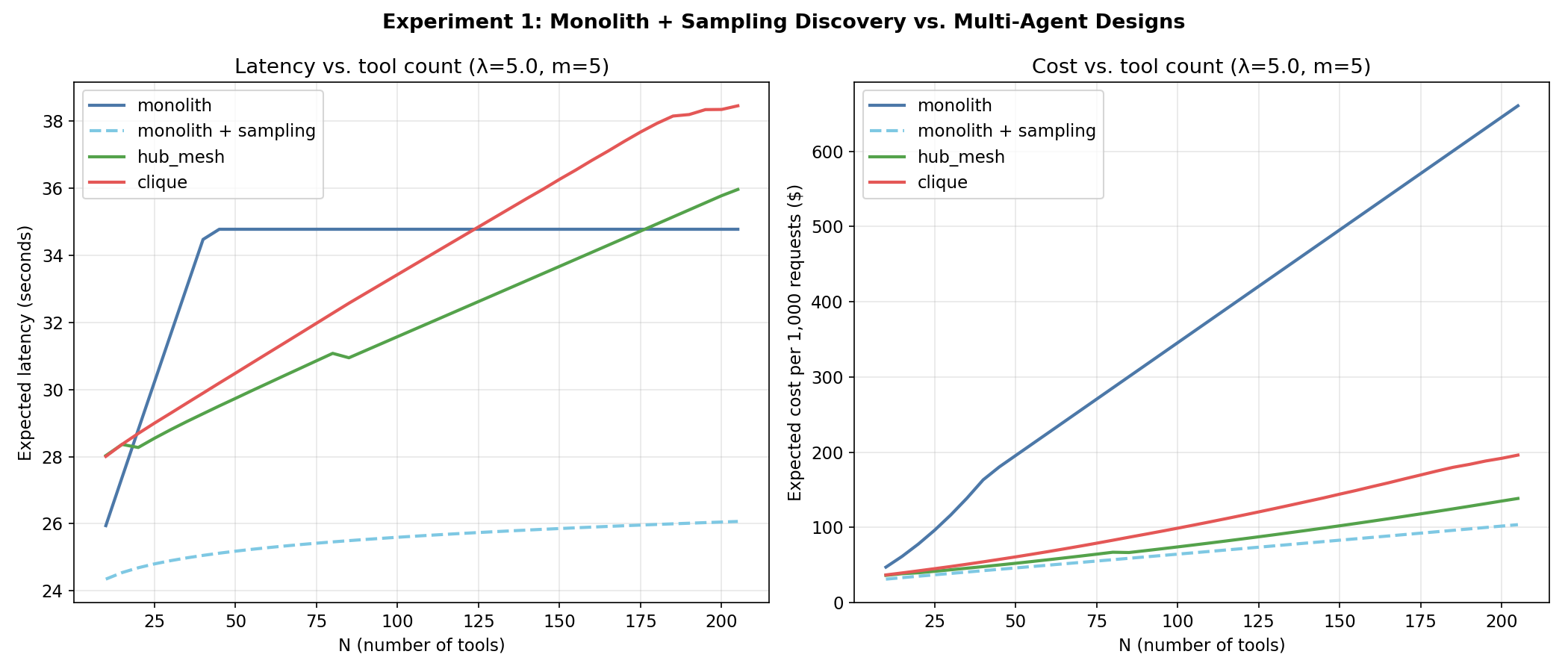
The results are clear:
- Latency: Monolith + sampling beats hub & mesh across the entire range up to . No crossover. The combination of zero boundary crossings and a tiny active scope gives it a persistent advantage.
- Cost: Monolith + sampling is also cheapest across the entire range. The context reduction from to is so dramatic that even the geometric retry overhead can’t offset it.
Experiment 2: How compact do summaries need to be?
I sweep the compression ratio from 0.05 (very compact, ~5 tokens) to 0.8 (barely compressed, ~80 tokens).
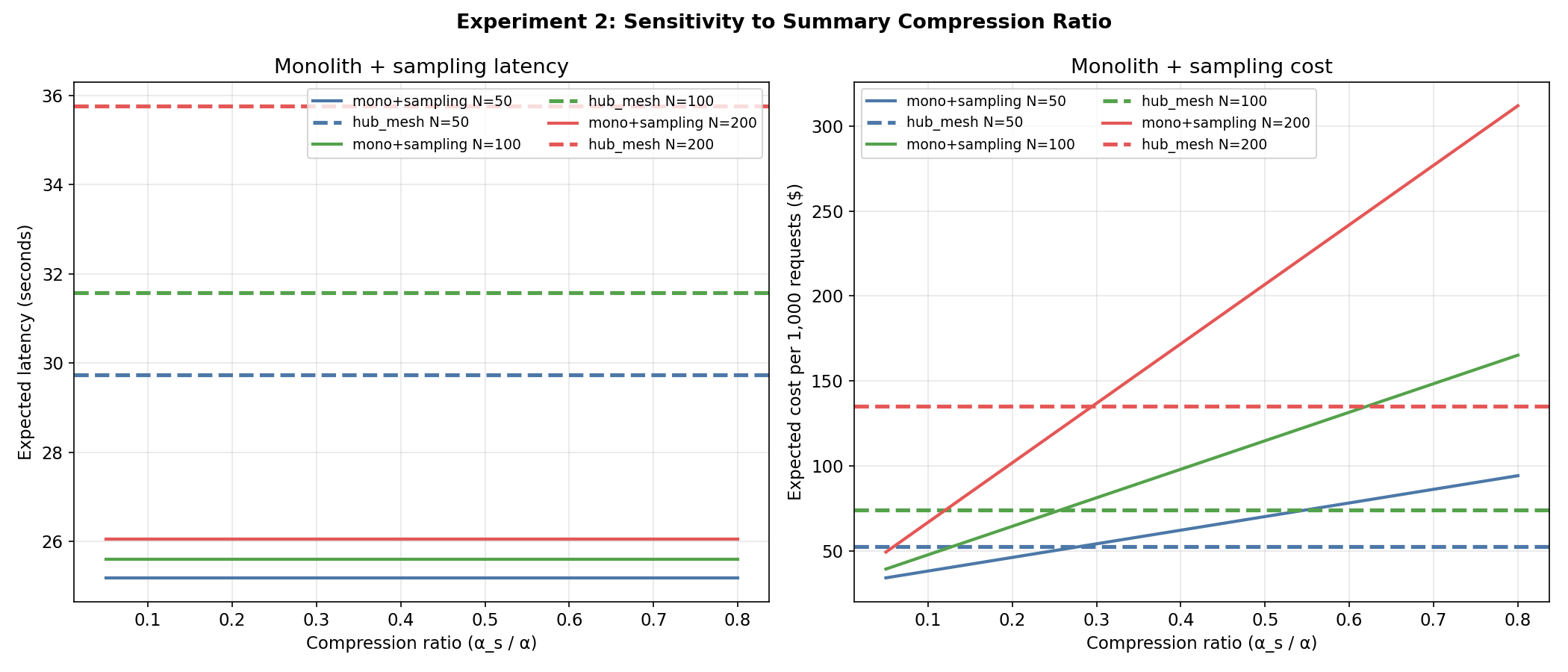
- Latency is robust to summary verbosity. The sampling monolith stays below hub & mesh baselines regardless of compression ratio. Latency is dominated by turns, and turns don’t change with .
- Cost is more sensitive. At high ratios, the cost advantage erodes. But even at 0.5, the sampling monolith remains cheaper for . In practice, a tool name and one-line description at ~20 tokens (ratio 0.2) is very achievable. (Or even one very long line… perhaps ~40 tokens.)
Experiment 3: How good does discovery need to be?
I sweep discovery error rate from 0 to 0.30.
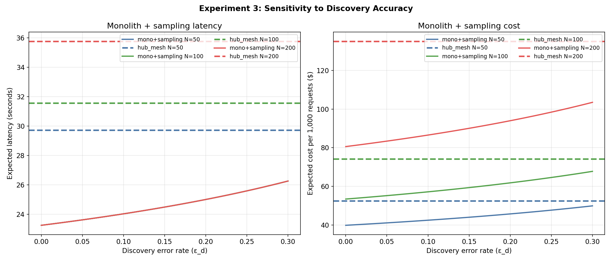
The sampling model is remarkably tolerant of discovery error. Even at a 30% miss rate, monolith + sampling remains both faster and cheaper than hub & mesh for all tested tool counts. Discovery errors only add geometric retries (a multiplicative factor on turns), while the context and choice-error savings are structural.
The practical implication: your discovery mechanism doesn’t need to be perfect. Even a mediocre semantic match is enough.
Experiment 4: How many tools should you load per attempt?
I sweep from 1 to 60. This is the most revealing experiment.
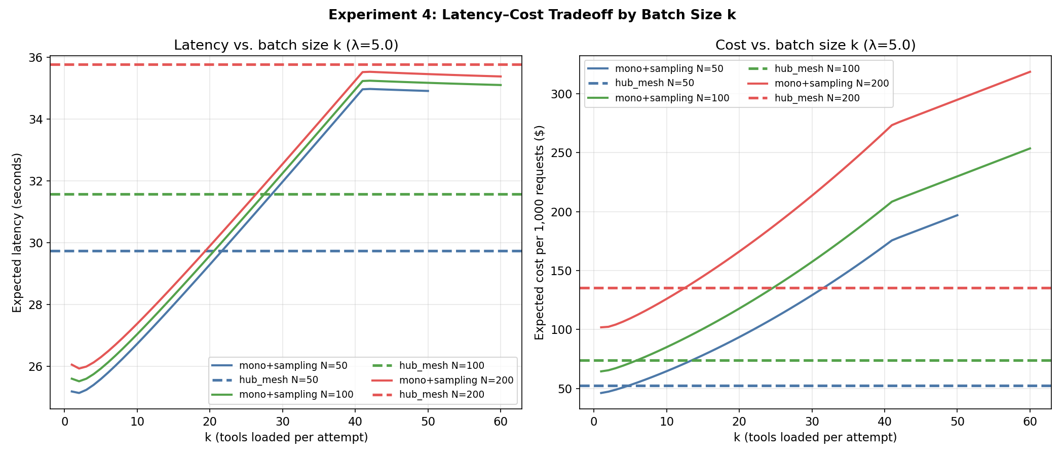
It exposes a clean latency-cost tradeoff:
- Optimal for latency: 2 (for all tested ). Moving to reduces discovery retries enough to offset the marginal increase in choice error. Beyond , the choice error term takes over.
- Optimal for cost: 1 (for all tested ). Cost is monotonically increasing in .
is the right default. It is the cheapest option and only marginally slower than . The “many cooks” effect from the original model is still in effect; it just kicks in at a much smaller scope.
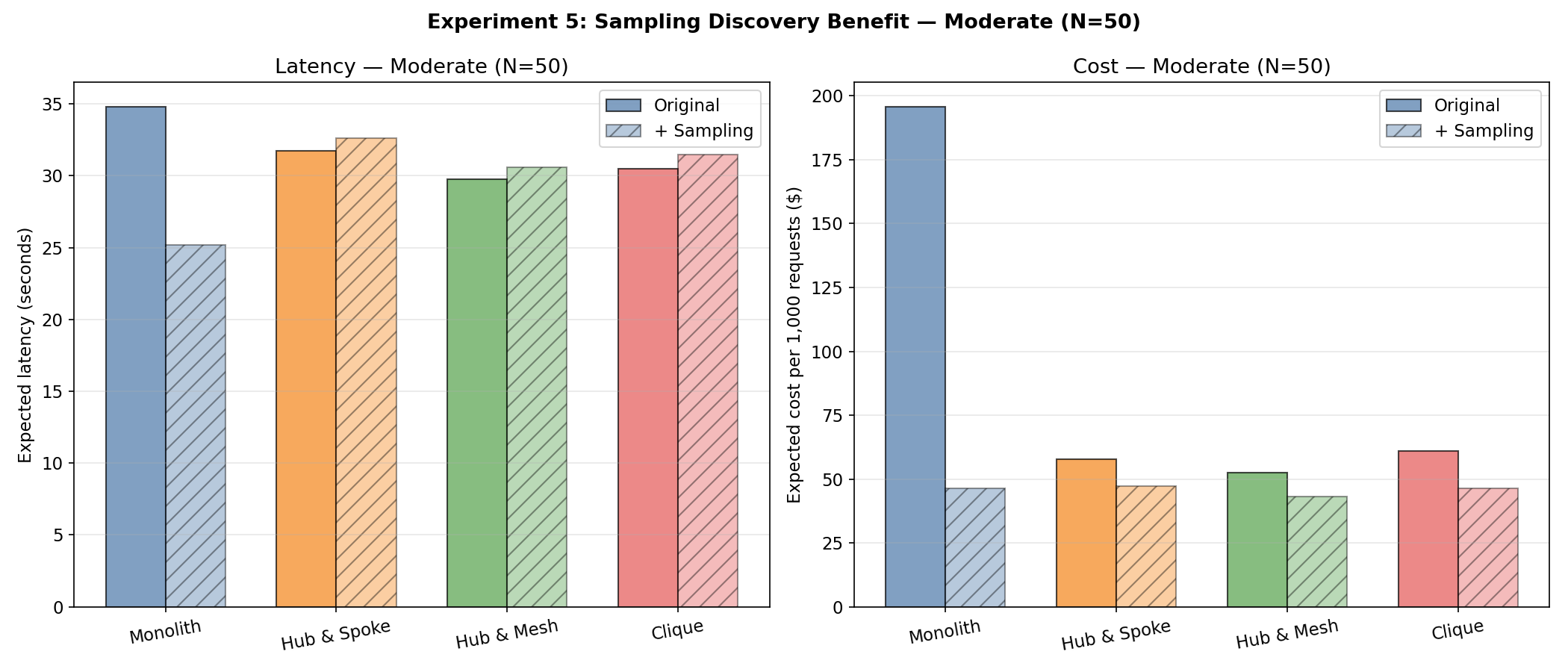
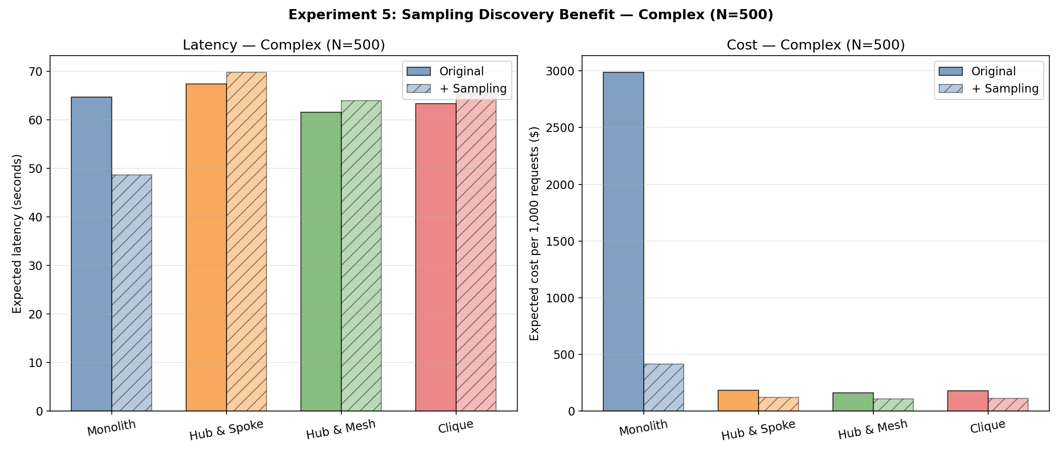
Experiment 5: Does sampling help multi-agent designs too?
I apply sampling to all four designs and compare before/after.
| Scenario | Design | Latency | Cost |
|---|---|---|---|
| Moderate () | Monolith | -27.6% | -76.3% |
| Moderate () | Hub & Mesh | +2.9% | -17.8% |
| Moderate () | Clique | +3.1% | -24.1% |
| Complex () | Monolith | -24.9% | -86.2% |
| Complex () | Hub & Mesh | +3.8% | -34.0% |
| Complex () | Clique | +3.5% | -36.9% |
The monolith benefits disproportionately. Multi-agent designs see a modest latency penalty (~3% from retries) but meaningful cost savings (18-37%), since sampling reduces their per-agent contexts too. The effect is smaller because their agents already had small scopes.
Experiment 6: Updated heatmaps
I re-run the (, ) heatmaps with monolith + sampling as a candidate.
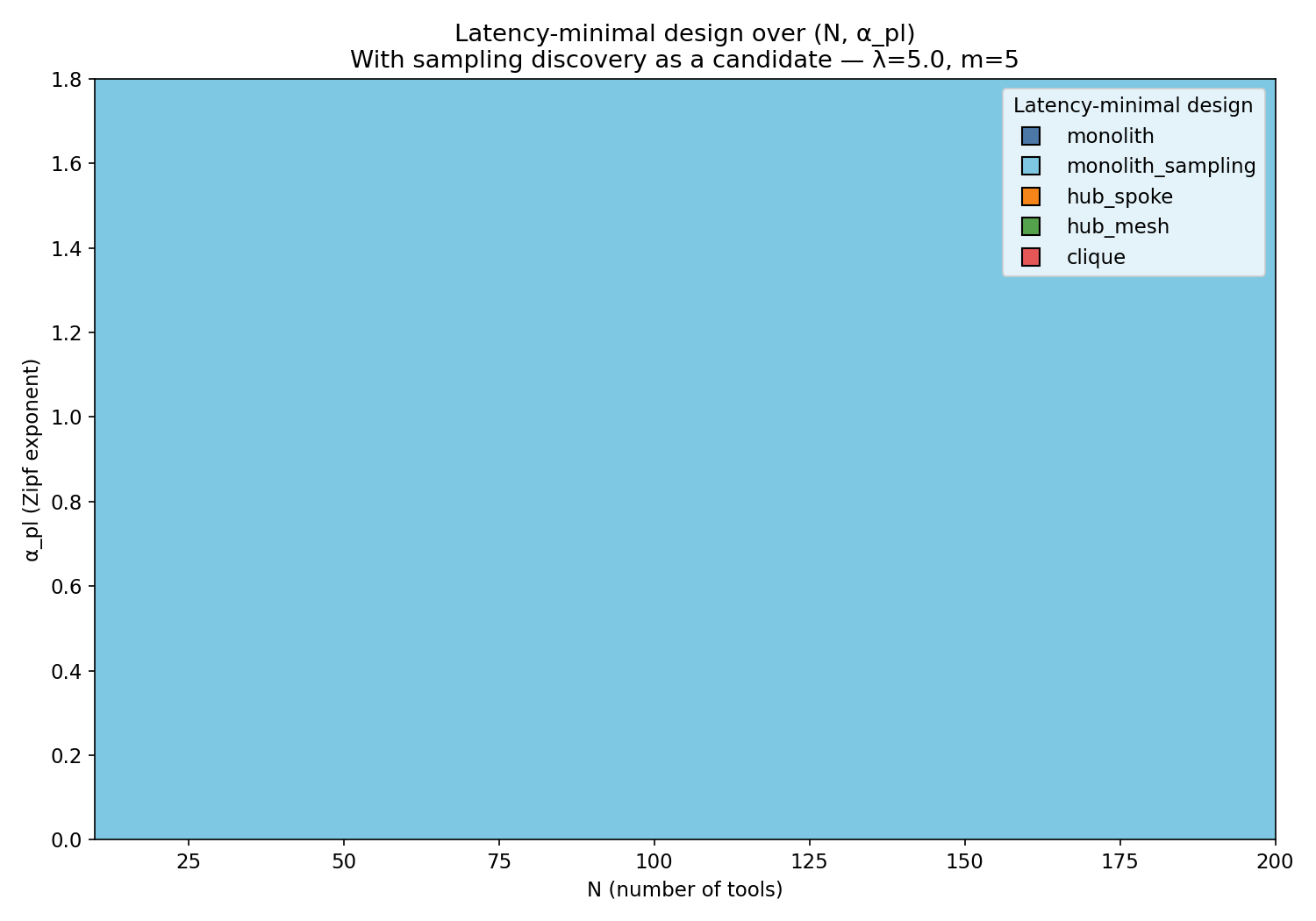
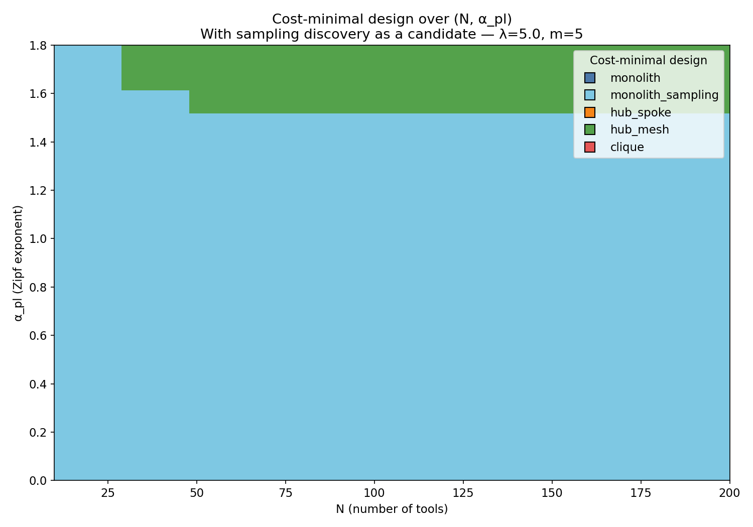
Both heatmaps are dramatically different from the original paper’s. Where hub & mesh and clique used to dominate, monolith + sampling now owns nearly the entire space.
6. What about token caching?
One thing that has been nagging at me since the original paper is token caching. If the LLM provider caches tool definitions across turns, the monolith’s per-turn cost and latency drop, potentially making progressive loading less necessary. Is the additional architectural complexity of progressive loading worth the savings, with cached rates in place?
Let us quickly try to model it…
The caching model
Most major providers now offer some form of prompt caching. Anthropic, for example, gives a discount of 90% for cached input tokens (albeit with a charge for cache creation, varying depending on whether you select a 5-min or 10-min cache TTL), with some amount of latency improvement for processing cached content. OpenAI charges a flat 50% rate for cached input tokens without a separate cache creation charge.
Note that if you’re not using the latest models via Anthropic’s first-party API, there are some complications e.g. you need to manually handle cache creation and TTL. I ignore those complications for this discussion.
With that in mind, I model the simple case conservatively:
- Cost: 90% savings on cacheable input tokens (you pay 10% of base price).
- Latency: no change to TTFT. This is the conservative floor. In reality a cache hit skips prefill on the cached prefix, so TTFT usually drops on every turn after the first; the first turn is a cache write, which leaves TTFT roughly unchanged. Assuming zero benefit keeps the comparison honest — any real caching system should do at least this well.
Two clarifications, since TTFT is easy to conflate here. (1) “TTFT” here means time-to-first-token of a single model call. The extra latency from an agent spending a discovery turn before it can answer is a turn-count effect, already captured in — I don’t double-count it in TTFT. (2) This analysis assumes the cacheable prefix is stable for the whole conversation. Anything that rewrites earlier context — compaction, context editing, tool-result truncation — invalidates the cache from that point on. I exclude those from the model; in a long, compaction-heavy session the cost savings below are an upper bound.
The key question is: what is cacheable? For any agent, the system prompt and tool definitions are (ideally) identical across turns within a conversation. They’re the perfect cache candidates. The conversation history and per-turn payload change and can’t be cached.
For each design:
| Design | Cacheable per turn | Non-cacheable per turn |
|---|---|---|
| Monolith | (all tool defs) | Payload, error context |
| Mono + sampling | (summaries) | (loaded tool changes each turn) |
| Hub & mesh | $L_0 + \alpha \cdot | S_i |
Results
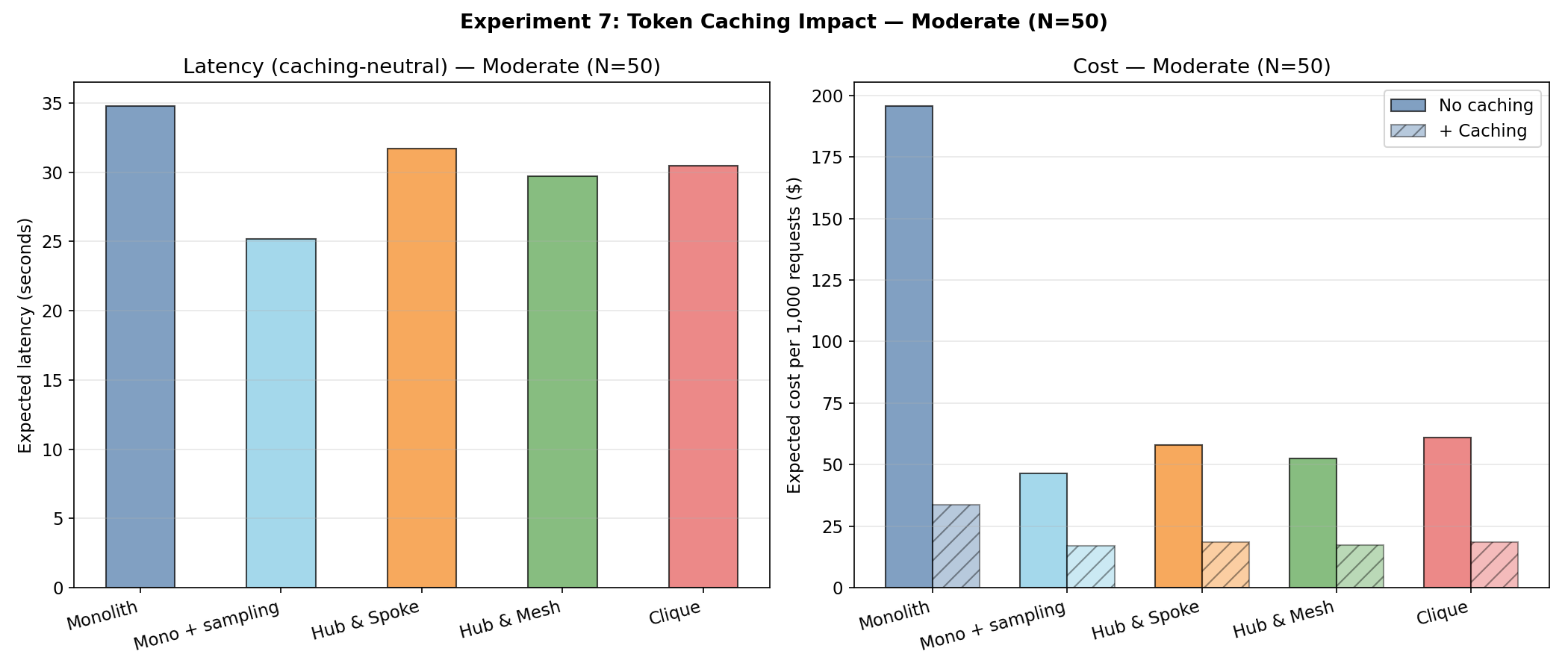
Here is what the numbers say for the moderate scenario (, ). Under the conservative assumption above, caching is latency-neutral, so latency is a single column; the cost columns show the before/after:
| Design | Latency | Cost per 1K requests | |
|---|---|---|---|
| No cache | + Cache | ||
| Monolith | 34.8s | $196 | $34 |
| Mono + sampling | 25.2s | $46 | $17 |
| Hub & mesh | 29.7s | $52 | $17 |
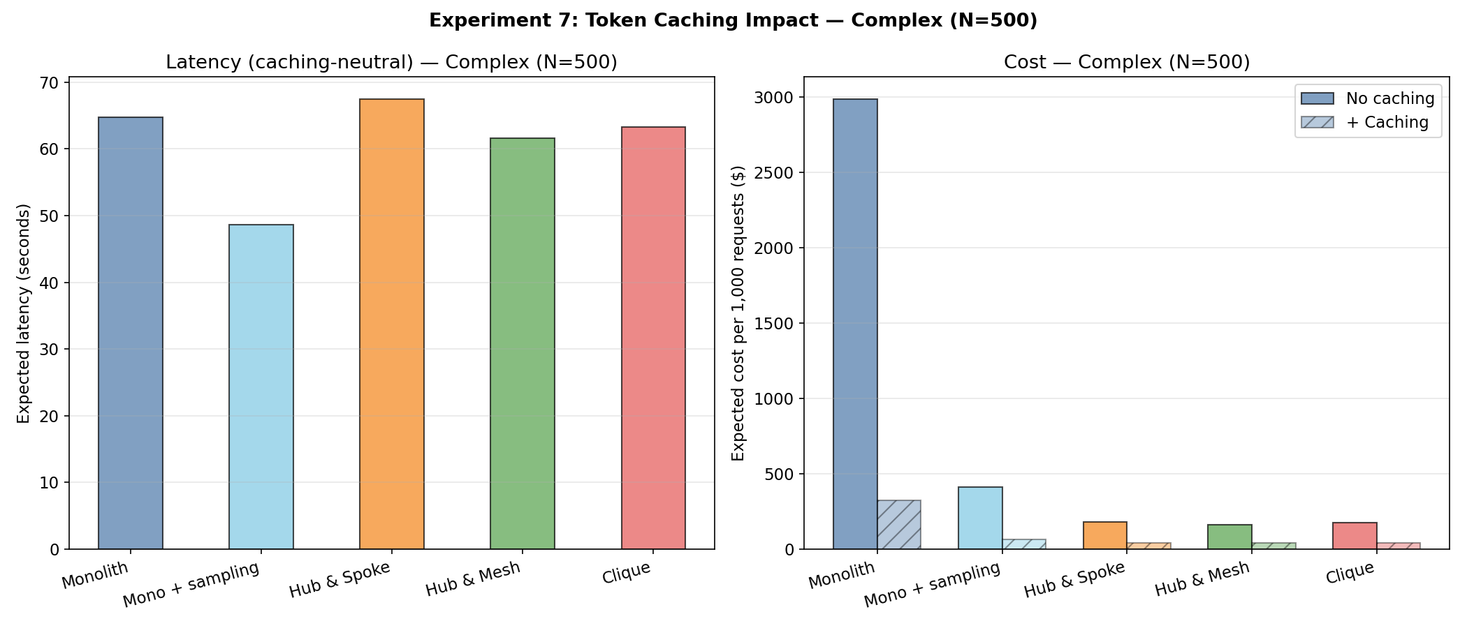
And the complex scenario (, ):
| Design | Latency | Cost per 1K requests | |
|---|---|---|---|
| No cache | + Cache | ||
| Monolith | 64.7s | $2,987 | $324 |
| Mono + sampling | 48.6s | $412 | $64 |
| Hub & mesh | 61.6s | $160 | $40 |
What this tells us
Three things jump out:
1. Caching narrows the cost gap but doesn’t close it (at moderate N). At , the sampling monolith and hub & mesh converge at ~$17 per 1K requests — both dramatically cheaper than the uncached monolith ($196). Caching helps the original monolith enormously (from $196 to $34), but it still can’t match the other two.
2. The sampling monolith maintains its latency advantage regardless of caching. Under the conservative model, caching is latency-neutral, so the ordering is unchanged: the sampling monolith at 25.2s still beats hub & mesh at 29.7s. This is because latency is driven by turns, and the sampling monolith has the fewest turns (8.2 vs. 11.4 for hub & mesh). Caching is a lever on per-turn cost, not on turn count — and to the extent a cache hit actually lowers TTFT, it lowers every design’s latency without changing their order.
3. At very high N, multi-agent designs can be cheaper with caching. At , hub & mesh + caching ($40) undercuts sampling monolith + caching ($64). This makes sense: the hub & mesh agents have tiny scopes (2-19 tools each), so their cacheable context is already small. The sampling monolith still carries 500 summaries.
The bottom line: token caching is complementary to progressive loading, not a substitute. The best option at moderate scale is sampling monolith + caching. At very large scale (500+ tools), you might want multi-agent + caching for cost, but the sampling monolith still wins on latency. And under the more realistic assumption that caching reduces TTFT (rather than increasing it), the sampling monolith’s latency advantage would be even larger.
7. How should agents discover tools?
The model assumes agents find tools by scanning an always-in-context directory of summaries. But that is not the only option, and at scale it might not even be the best one. Here are three discovery strategies and how they map to the model.
Strategy 1: Tool directory (always in context)
This is what the current model assumes. All tool summaries live permanently in the agent’s context, costing tokens per turn.
How it works: The agent sees a flat list of (name, description) pairs. When it needs a tool, it scans the list and requests one by name. If it picks wrong ( probability), it retries.
Strengths:
- Zero-overhead discovery — no extra tool calls, no retrieval latency
- Deterministic: the agent always has the full picture of what is available
- Works out of the box with any function-calling model
Weaknesses:
- Context cost grows linearly with . At and , that is 10,000 tokens of summaries alone
- Discovery error scales with : harder to pick the right tool from a longer list
- Stale context: the same summaries sit in every turn whether or not they’re relevant
Best for: . This is the regime where the context cost is manageable and the discovery error is low (~22% at ).
Strategy 2: Grep-style search
Instead of keeping all summaries in context, the agent calls a search tool that returns matching tools by keyword or pattern.
How it works: The agent formulates a search query (e.g., “file editing tools”), and a retrieval function returns the top- matching summaries. The agent then picks from those candidates.
Real-world example: Claude Code’s ToolSearch works exactly like this. The agent knows deferred tools exist but only sees their full definitions after searching for them by keyword. Coding agents commonly use this pattern for navigating large codebases — the same logic applies to navigating large tool sets.
Model implications:
- Context per turn drops from to (where , typically 3-5 results)
- But each discovery attempt now costs an extra turn (the search call itself), so the effective retry cost is higher
- Discovery error depends on search quality: how well does the agent formulate queries, and how descriptive are the tool names?
Strengths:
- Context scales with , not — viable even at
- Forces the agent to articulate what it needs, which can improve precision
Weaknesses:
- Adds a turn of overhead per tool discovery (the search call)
- Discovery accuracy depends on the agent’s query quality and the tool naming conventions
- Keyword matching can miss tools with non-obvious names (e.g., the tool for “renaming files” might be called
mv)
Best for: , or rapidly growing tool sets where you don’t want to recompute the summary context.
Strategy 3: Semantic search
Like grep-style search, but using embedding similarity instead of keyword matching.
How it works: Tool descriptions are pre-embedded into a vector store. The agent’s request (or a description of what it needs) is embedded and compared via cosine similarity. The top- matches are returned.
Model implications:
- Same context savings as grep-style ( per turn)
- Potentially lower for ambiguous or synonym-heavy tool sets (semantic similarity captures “rename” ↔ “mv” better than keyword match)
- Higher infrastructure cost: requires an embedding model, a vector index, and a retrieval pipeline
Strengths:
- Handles synonyms and natural-language descriptions well
- Can surface tools the agent wouldn’t think to search for by keyword
Weaknesses:
- Semantic similarity ≠ correct tool. A “semantically close” tool might do something subtly different
- Embedding quality matters: if tool descriptions are poor, embeddings will be too
- Infrastructure overhead: embedding model, vector store, retrieval pipeline
Best for: Large with high semantic overlap between tools, or when tool descriptions are natural-language rather than structured.
The hybrid: hot cache + search
In practice, we would probably combine approaches. For example, we could keep the top- tools always loaded (by Zipf mass) and use search for the long tail. Under Zipf(), the top five tools often cover ~half of all requests. Those tools should always be in context — they’re too popular to pay the search overhead for. Everything else gets discovered on demand.
This maps naturally to the model: the “hot cache” is a small directory ( tokens), and the long tail is discovered via search. The discovery error for hot tools is near-zero (since they’re always available), and the error for tail tools follows the search mechanism’s .
I haven’t modeled this hybrid formally, but it is a natural extension and likely the right production architecture.
Two refinements could make this even more powerful in practice.
Keep a few tools fully loaded, not just summarized. The hot cache doesn’t have to stop at summaries. For a handful of ubiquitous, high-reliability tools it is worth keeping the full definition permanently in context. The canonical example is a shell/Bash tool: coding agents typically keep one always available, and because models are already extremely fluent with the shell, its discovery and choice error are effectively zero. An always-on Bash tool also substitutes for a long tail of niche tools — grep, file reads, small scripts, one-off munging — which shrinks the effective the discovery mechanism has to cover. A reliable general-purpose tool is worth more than its one slot suggests.
Discovery amortizes over a conversation. The sampling model charges full discovery cost on every tool call, but in a real session the same tool often gets used repeatedly. Once discovered and loaded, keeping a tool resident makes every subsequent use free of discovery cost — so the per-call tax is an upper bound. Long conversations with tool reuse pay less than the model assumes, which again pushes in the sampling monolith’s favour.
8. Discussion
What changed from Part 1?
The original paper’s core tension was: the monolith is fast (no boundary crossings) but expensive (huge context, high error rate). Multi-agent designs traded speed and architectural simplicity for cost savings and fewer errors.
Progressive loading breaks this tradeoff on two fronts:
-
Context reduction. Per-turn context drops from to . For : from 6,000 to 2,080 tokens. For : from 51,000 to 11,080.
-
Choice error elimination. By keeping the active scope to , the “many cooks” problem vanishes. Choice error drops from ~0.9 to ~0.08 at , eliminating the monolith’s biggest source of wasted turns.
The second effect is the more important one. It makes the sampling model qualitatively different from a batch-loading approach: batch loading still requires the agent to select from loaded tools (where ), preserving a non-trivial choice error. Sampling at eliminates this — there is only one tool loaded, so there is no choice to make.
More caveats
Here are a few other issues that could significantly change design recommendations from this article.
The choice error model amplifies the result. With and , the original monolith hits the 0.9 ceiling. If choice error scaled more gently with scope (say, logarithmically instead of linearly), the gap between original and sampling monolith would be smaller. We need empirical measurement of how tool mischoice actually scales with scope.
Token caching matters, but doesn’t affect turn count. As shown in Section 6, caching narrows cost gaps but preserves the turn-count hierarchy. The sampling monolith still wins on latency. At very high (500+), multi-agent + caching can be cheaper, but that is a niche regime.
The “one tool per turn” assumption persists. In practice, agents often call multiple tools in parallel. This would require loading tools simultaneously, which (per Experiment 4) starts reintroducing choice error. Parallel tool calls would narrow the gap between designs.
Discovery accuracy is hand-waved. (Well everything in this article is hand-waved, but this one is even more so!) The default gives ~22% error at , which feels realistic but hasn’t been empirically validated. Different discovery mechanisms (directory vs. grep vs. semantic search) would produce different profiles, as discussed in Section 7.
No empirical validation yet. These are still analytical results from a model with many assumptions. We should validate this against real workloads. While I’ve built a number of agentic systems, including multi-agent ones, and talked to many people who have also done the same, that is different from empirically (and rigorously) measuring/estimating some of these parameters and seeing whether or not the model is even a good fit.
The harness matters as much as the architecture. This model treats the agent as a bare model + tool loop, but production systems run inside a harness — the scaffolding that decides how tools are presented, how results are truncated, when to retry, when to compact, and whether calls run in parallel. These harnesses are becoming increasingly sophisticated. A good harness affects almost every constant here: tighter summaries lower , better formatting and naming lower , smarter retry logic changes the error penalties. Much of the recent step-change in coding agents came from harness improvements, not just stronger base models. So read these results as directional given a fixed harness — a better one can widen the sampling monolith’s lead, and a clumsy one can erase it.
Revised design recommendations
The original paper concluded: “Always start with a monolith, then move to hub & mesh or clique.” Here is the updated version:
-
Start with a monolith + progressive tool loading. This is now both the fastest and cheapest design across virtually the entire parameter space we tested (). The monolith is back — not by brute-forcing a massive context, but by being smart about what is in context at any given moment.
-
Use as the default. Pure sampling (one tool at a time) is cost-optimal and near latency-optimal. Only consider if you’re strictly latency-constrained.
-
Multi-agent designs are no longer the default for cost. The case for multi-agent is now primarily organizational (different teams own different agents), architectural (different model configs per agent), or operational (isolation between failure domains) rather than economic. At very large (500+), multi-agent + token caching can be cheaper — but even then, the sampling monolith is faster.
-
Discovery accuracy barely matters. Even a 30% miss rate doesn’t change the qualitative conclusion. Don’t over-invest in a perfect discovery mechanism at the expense of shipping.
-
Combine progressive loading with token caching. They’re complementary: progressive loading reduces turns and scope; caching reduces the per-turn cost of whatever context remains. The combination is the cheapest option at moderate scale. Just make sure your agent’s prompts are cacheable, i.e. no dynamic tokens within the first N tokens depending on your model’s cache parameters.
9. More practical recommendations
If you are building an agent, here are a few more practical tips:
Writing good tool summaries
Your summaries need to answer one question: when should this tool be used? Not how it works, not what parameters it takes — just when.
A good summary for a file-editing tool:
Edit: Make targeted replacements in existing files. Use when modifying specific sections of code.~20 tokens. That is enough for the agent to decide “yes, I need this” or “no, I need something else.”
A bad summary:
Edit: Takes file_path (string, required), old_string (string, required), new_string (string, required), replace_all (boolean, optional, default false). Performs exact string replacements in files using a diff-based approach.That is ~40 tokens and most of it is parameter detail the agent doesn’t need until it is actually calling the tool.
The discovery loop in pseudocode
def agent_turn(user_request, tool_summaries, conversation):
    # Agent sees: system prompt + all summaries + conversation
    # Agent decides it needs a tool
    tool_name = llm_pick_from_summaries(tool_summaries, user_request)

    # Load the full definition
    tool_def = load_tool(tool_name)

    # Agent now sees: system prompt + all summaries + this one full def
    result = llm_call_tool(tool_def, user_request, conversation)

    if result.wrong_tool:
        # Retry: pick a different tool from summaries
        return agent_turn(user_request, tool_summaries, conversation)

    return result
Choosing a discovery strategy
| Your situation | Recommended discovery | Why |
|---|---|---|
| < 50 tools | Full definitions, no progressive loading needed | Context cost is manageable; don’t add complexity |
| 50-200 tools | Tool directory (always in context) | Sweet spot: summaries are cheap, discovery error is low |
| 200-1000 tools | Grep-style search | Summary context starts to bloat; search keeps it bounded |
| 1000+ tools | Semantic search or hybrid (hot cache + search) | Keyword matching breaks down at this scale. (Also, do you really need a single agent with so many tools??) |
When to go multi-agent anyway
Progressive loading doesn’t eliminate all reasons for multi-agent architectures. Consider splitting if:
- Different teams own different tools. Independent agent deployment, tool versioning, and on-call rotation sometimes matter more than token economics.
- Different tools need different models. Your coding tools might need Claude Opus; your search tools might be fine with Haiku. A monolith forces one model for everything.
- Isolation is critical. If a tool failure in one domain shouldn’t affect another domain, separate agents provide fault isolation.
- You’re at with strict cost constraints. As the caching analysis shows, multi-agent + caching can be cheaper at very large scale.
Remaining open questions
- Empirical validation. Real-world measurement of discovery accuracy, choice error scaling, and the interaction between caching and progressive loading. This is the biggest gap.
- Parallel tool calls. How does loading interact with agents that naturally batch tool calls? The model suggests it reintroduces choice error, but the magnitude needs measurement.
- The hot cache variant. Formally modeling the “always keep top- loaded + search for the rest” hybrid.
- Cross-model generalization. These results use GPT-4.1 pricing and latency. Different models have very different cost structures and context limits.
- The skill composition problem. If skills bundle tools with prompts and examples, how does progressive loading interact with skills that depend on each other? Loading one skill might require context from another.
The simulation code used for this analysis is on GitHub at ycmak/agentic-design-patterns, alongside the original notebook. (Thanks to Claude for helping me implement the code based on the mathematical model I sketched out.)
*This post extends the original analysis from October 2025. If you have empirical data on progressive loading or tool discovery in production agent systems, I’d love to hear from you on LinkedIn!